
12. Algorithms
In this chapter we explore searching and sorting algorithms.
One way to analyze an algorithm is to think about its performance as the size of the input data increases.
The chapter also contains some exercises to explore searching and sorting algorithms.
Searching
Linear search
We have already explored how to find an item in a list. We search for the value of interest by iterating through the items in the list and checking each one. This is called “linear search”. In general, to find an item in a list of length \(n\), we need to make at most \(n\) comparisons. Mathematically we say “linear search is \(O(n)\)”, where the “big O” notation indicates an upper bound for the number of computations.
In general, we say an algorithm is \(O(f(n))\) if the number of computations is at most a constant multiple of \(f(n)\) as \(n\) gets large. In other words, \(k f(n)\) is an upper bound for the number of computations for some \(k\), for large \(n\).
Because the graph of \(f(n) = n\) is a line, if an algorithm is \(O(n)\), we say it is “linear in time complexity”. If an algorithm is \(O(1)\), the number of computations is bounded by a constant, and we say the algorithm has “constant time complexity”.
Binary search
When you search for a word in a dictionary, you do not need to compare every word in the list. Because the dictionary is sorted, you can compare to a word in the middle, and then choose which half of the dictionary to continue your search. Then you do the same thing in the smaller list: you compare to a value in the middle, and choose which half to search next.
In each iteration, the size of the list to search is reduced by half, eventually resulting a list with a single item for a final comparison. For example, in a list with 8 items, binary search will take 3 iterations, because \(2^3 = 8\). In a list with 1024 items, binary search takes 10 iterations, because \(2^{10} = 1024\). In general, for a list with \(n\) items, binary search will take \(\log_2{n}\) iterations. In other words, binary search is \(O(log(n))\), or “logarithmic in time complexity”. (Note that because all logarithms are multiples of each other, we can omit the subscript from the big O notation.)
Sorting
As we have seen above, binary search is much more efficient than linear search (logarithmic vs. linear time complexity). Because of this, it is advantageous to work with sorted data. There are many different sorting algorithms, with different time complexities.
Selection Sort
Here is the algorithm for selection sort:
- find the smallest element in the input list
- remove it and add it to the output list
- repeat until the input list is empty
Assuming that adding or removing an element from a list is constant time, the algorithm consists of multiple linear searches with decreasing number of elements: \[ n + (n-1) + \ldots + 2 + 1 \] This sum is given by a formula \[ \dfrac{n(n+1)}{2} \] which is bounded by \(k n^2\) for some \(k\), so selection sort is \(O(n^2)\) (quadratic).
Insertion Sort
Insertion sort is similar to how a card player sorts her hand as the cards are being dealt from the dealer.
For each item in the input list:
- find correct position in the sorted output list
- insert the item
Finding the correct position to insert an item into a sorted list
is \(O(n)\), similar to linear
search:
\[
1 + 2 \ldots + (n-1) + n
\] so insertion sort is also \(O(n^2)\).
Merge Sort
Merge sort is a divide-and-conquer algorithm:
- split list into two halves, and sort each half
- merge the two sorted halves
In the first step, “sort each half” can be thought of as a recursion, where these same two operations are performed on each half. Similar to binary search, the “bottom” of the recursion is a single item, which is trivially sorted.
The core of the algorithm is the merge operation, which takes two sorted lists and merges them into a single sorted list:
- examine the top item from each of the two input lists
- remove the smaller item, and add it to the output list
- repeat until both input lists are empty
The merge operation involves \(O(n)\) comparisons. Because the lists are divided in half each time, there are \(O(\log n)\) merge operations. So the time complexity is \(O(n \log n)\), or “log-linear”.
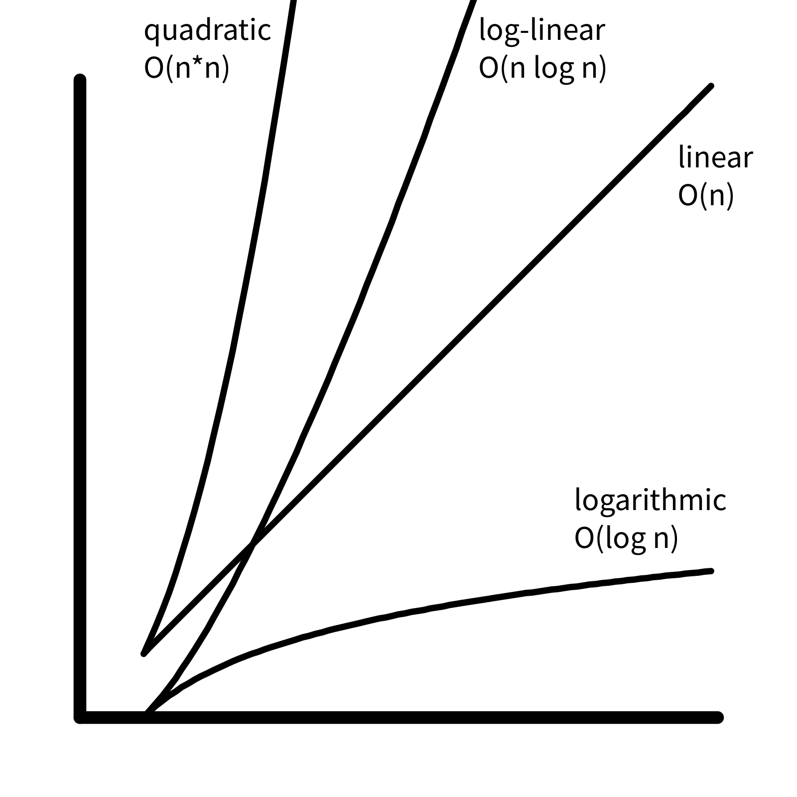
Time complexity comparison